An automated analysis of the optic nerve

Michel Matter & Jean-Marc Matter

contacts : michel.matter@gene-vision.ch, jean-marc.matter@gene-vision.ch

Context

The human optic nerve connecting the retina to the visual area of the brain is made of about one million axons. In birds, this number can reach several millions. The optic nerve remains from many sides a terra incognita due to the difficulty of its study in primates. However, birds can help us to answer several key questions. Axons of ganglion cells (GC) constitute the optic nerve and are responsible for transmitting the visual information, encoded as a nerve signal, from the retina to the brain. Counting these axons on slices of the optic nerve is currently one of the most reliable available methods for knowing the number of GC present in the retina.

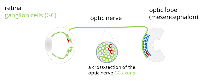
A figure showing the retina and the connection via the optic nerve to the optic lobe — Illustration of the principle of how a visual signal is transmitted from the retina to the brain according to a retinotopic mapping : neighboring ganglion cells in the retina (in red) have axons that remain close to each other in the optic nerve and which activate neighboring cells in the optic lobe.

Axons are organized in the optic nerve according to a so-called retinotopic mapping which produces a homeomorphic representation of the visual field in the brain. In other words, any image caught by the eye and sent to the brain suffers only from continuous deformations – imagine a picture printed on an elastic membrane, e.g. a balloon, and suppose that the image can be deformed by bending, folding or twisting the membrane but never by ripping it. Any two points located next to each other on the initial picture will remain next to each other during the whole mapping process until the picture is projected in the brain.

Counting axons and analysing their sizes as well as their distribution in the optic nerve provide thus information about the number and the distribution of ganglion cells of different types, such as midget (called P-GC) and non-midget (called M-GC or parasol GC) ganglion cells.

Goals

Performing a morphometric analysis of the optic nerve requires to identify all axons composing it, in order to study their number, their sizes, their shapes and how they are organised. We thus need to detect each visible axon on a microscope picture by precisely identifying its contour. Given the enormous number of axons, performing this task entirely manually would be excessively long and tedious. Our aim is thus to develop a way to achieve this automatically.

A figure showing the photography of an entire section of an optic nerve. A regular grid is drawn on the photography, dividing the whole section into square tiles. In the right part, a zoom over a single tile is shown. One sees a great number of axons on this zoomed image. — Left : an entire section of an optic nerve coming from a barn swallow (*Hirundo rustica*) is about 1 mm diameter large (image made with an optic confocal microscope) ; right : zoom on a 0.05 mm x 0.05 mm portion. Such portions will serve as a basis for the axon detection algorithm.

Approach

We plan to apply deep learning algorithms using an approach called image segmentation. Image segmentation is an example of supervised learning : one first shows to the algorithm a sequence of images labeled manually – the training set. An example of such a labeled image is shown below :

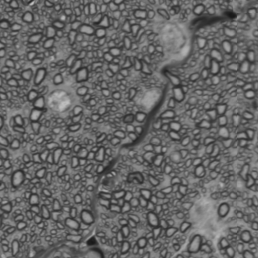
A photography showing a portion of an optic nerve section. One sees a lot of circular shapes corresponding to the axons — A portion of an optic nerve section

An image in two colours showing a profusion of approximately circular white shapes on a black background — Segmentated image – a black and white mask with axons highlighted in white. This mask was produced by manually annotating each visible axon, in order to serve as a training example for the algorithm.

The manual annotation consists here in preparing a binary (black and white) mask which marks the objects that should be detected by the algorithm. The algorithm is then going to learn how to reproduce the most accurately possible each of the binary masks in the training set by using only features from the original images – this is the training phase. A successful training will allow the algorithm to generate accurate binary masks from new images that it hasn’t seen before – this is the prediction phase.

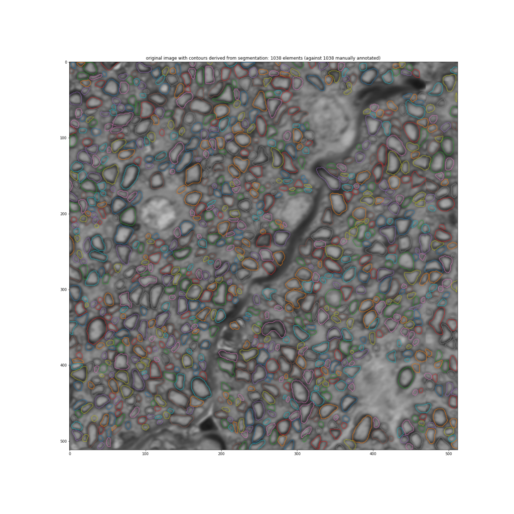
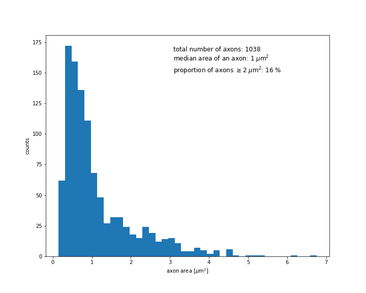
Then, from a binary mask as the one shown above, it is not difficult to automatically identify the contours of the axons in order to study their sizes, their shapes and their organization within the optic nerve. This is shown in the following figure :

A photography of an optic nerve portion. The contours of the axons are highlighted using different colours — The same portion of the optic nerve section as before but with axon contours highlighted. The highlighting was performed automatically from the corresponding binary mask.

An histogram showing the distribution of the axon areas for a portion of the optic nerve — Example of a morphometric analysis : distribution of the axon areas on this portion

The algorithm that we use for predicting binary masks from true images is a so-called convolutional neural network (CNN). A neural network is a mathematical construction organized in layers. The task of each layer is to detect different geometrical shapes. Every layer is made of units called “neurons”. Neurons from neighboring layers are connected to each other so that the information received from upstream layers and processed by a given layer is propagated to layers downstream. A given neuron activates if the incoming signal coming from neurons located upstream exceeds a given threshold. It then sends this activation signal downstream.

The first layers of the CNN learn how to detect simple geometrical shapes such as vertical or horizontal edges, whereas layers located deeper inside the network keep track of the information from all previous layers and use it to learn how to detect more complicated shapes. In this way, the network learn how to detect and localize in the image the elements that should be detected.

Challenges of this approach

The challenge of building and training a successful neural network is two-fold : one has to design the architecture of the network, i.e., the number of layers, the way they are connected to each other, etc., that is suited to the task. Then, one must provide the algorithm with a training set of manually annotated images that is large enough so that the algorithm can learn how to generalize, that is, accurately generate binary masks from new images that it hasn’t seen before.

The required amount of images for an efficient learning depends on the size of the neural network as well as on the kind of images that are targeted. It can vary from dozens to thousands. Settting up a training set that is large enough can thus be a long and tedious task. However, techniques of data augmentation that allow to reduce the size of the training set exist and are extensively used, especially in the domain of bio or medical imaging where the number of manually annotated images is often limited (sometimes a few dozens only). Such data augmentation techniques consist in reusing each hand-annotated image several times by slightly modifying it through geometrical transformations such as rotations, translations or distorsions.

We plan to start with an existing network architecture called U-Net ( arXiv:1505.04597 ) that has been developed for biomedical image segmentation. However, as biomedical images differ a lot depending on their nature, adaptations of the initial architecture will be probably necessary in order to accurately capture the morphological specificities of the optic nerve. We are also preparing a training set of manually annotated images that is large enough in order to train the network efficiently. In addition of that, we are going to rely on data augmentation techniques in order to amplify this set and optimize its use.

Preliminary results

Preliminary results of training the neural network on a set of eight manually annotated images only, but amplified with a data augmentation technique are promising, as shown below :

A figure in four parts comparing a manual annotation (top) of the axons versus an automatic one (bottom). — top: a binary mask constructed manually and axon contours automatically highlighted from this mask ; bottom : a binary mask generated by the neural netwok algorithm from the same image and axon contours automatically highlighted from this mask.

Further steps will consist in increasing the size of the training set. We will then focus on the network architecture as well as on parameter tuning with the aim of optimizing the network performance.